Positive and Negative Reviews About Heaven Is for Real
Sentiment analysis in conjunction with motorcar learning is often employed to gain insight into how positive or negative a target group feels almost a particular entity, such as a movie, production line or political candidate. The key method to uncovering this is collecting samples of text from the target group (exist it tweets, client service inquiries, or, in this tutorial's case, production reviews). Information technology is a key part of natural language processing. This tutorial will guide you through the step-past-step process of sentiment analysis using a random woods classifier that performs pretty well. We will employ Dimitrios Kotzias'south Sentiment Labelled Sentences Data Ready, hosted past the Academy of California, Irvine. It contains picture show reviews from IMDB, eating house reviews from Yelp import and production reviews from Amazon. This guide volition elaborate on many fundamental machine learning concepts, which you tin then apply in your next projection. If y'all follow along with the code examples, you volition take a very useful, insightful (and fun) new technique at your disposal. This tutorial is divided into the post-obit sections: Auto learning and data science tin get complicated very fast: car learning algorithms are often long and convoluted, and organizing data in a reliable way tin become a headache. Fortunately, much of the groundwork is already established via Python libraries. Using these libraries, you can build, train, and deploy a neural network in a few lines of code, rather than hundreds. To make things easier on ourselves, we'll be using a number of libraries: If, while following along with the lawmaking, y'all try importing ane of these modules and receive an error, ensure the module has been installed by typing Alternatively, you can use a distribution of Python such as Anaconda, which will have many of these libraries and more than pre-installed. All this being said, I recommend you have some fourth dimension later to try doing some of these things from scratch, particularly, writing the code for some motorcar learning algorithms (neural networks and decision copse, for example). Don't worry well-nigh doing this just yet - for now, this tutorial will suffice. Annotation that nltk's stopwords listing may not come up pre-downloaded with the bundle. If you take trouble importing the stopwords list, blazon this once into a Python shell or type this in your Python file: We will exist using Dimitrios Kotzias's Sentiment Labelled Sentences Information Set, which y'all tin can download and excerpt from here here. Alternatively, yous can get the dataset from Kaggle.com here The dataset consists of 3000 samples of client reviews from yelp.com, imdb.com, and amazon.com. One-half of them are positive reviews, while the other one-half are negative. You can read more about the data set at either of the posted links. Once you've downloaded the .zip file and extracted the contents to a location of your choosing, you'll need to read the three .txt files in the "sentiment labelled sentences" folder into your Python session/IDE. (If you're looking for a lightweight, convenient editor that'southward used past many data scientists, I recommend Jupyter, which comes pre-shipped with Anaconda Navigator). Offset we read the information into Python: Now that nosotros take the information loaded in the Python kernel, we demand to format it into a usable structure. We at present take a listing of the form This list structure is a good first, but it has the potential to get messy as we interact with the data. Let's transfer the data to a pandas DataFrame, a data-structure with a well-organized format and many useful methods and attributes. This is one of the virtually popular data analysis packages in Python, often used by data scientists that switched from STATA, Matlab and and so on. By now, the content of those text files should await something similar this: With our data well-organized, we can start with the actual sentiment analysis and content classification. Before you start throwing algorithms at our corpus, information technology might assist if nosotros take a pace back and recall about patterns that we can see in the data. Doing this before nosotros spring into the machine learning volition help united states choose an effective strategy from the get-go, and not waste matter time on things that don't matter. We are ultimately interested in finding differences between negative and positive reviews - this is what our classifier will be doing, after all. Since we're dealing with text, some proficient places to look might include Nosotros'll consider each of these for both negative and positive classes, and compare the stats. Outset, lets compute some of this data using list comprehension and add it to our DataFrame. Now we accept Nosotros can apply the DataFrame'south built in statistic methods to get a summary of each of the new columns. Let'due south wait at some of the summary statistics. Continuing in that style: These statics signal that that there aren't huge divergence betwixt the classes - as far as these features go, negative and positive samples are pretty much the same. Let'southward see if we can spot any differences in the word selection present in either category. We'll mensurate term frequency using Python's Counter method, taken from the collections library. First, we'll demand to preprocess our data a chip. Due to the high frequency of words such as "the" and "and", nosotros demand a mode to view top word counts with these words removed. The nltk library has a pre-made list of common loftier frequency words, known equally stopwords. Nosotros'll import that list now. We tin now access a pre-made list of stopwords via And at present the negative form: Correct away, we can spot a few differences, such as the heavy use of terms like "skillful", "great", and "best" in the positive course, and words like "dont" and "bad" in place in the negative class. Additionally, if you increase the value of the n_most_common parameter, you tin encounter words like "not" (which nltk'southward corpus classifies every bit a stopword) in use five times as oftentimes in the negative class every bit in the positive form. Later spending a few minutes examining some trends in the data, we can proceed to build a model with some idea of what to focus on, and what not to. A uncomplicated classifier that merely focuses on word pick seems promising. We've come up a long way, and we're now most ready to start building our classifier. Before doing so, nosotros need to translate our textual data into a form the computer tin can empathise. This is commonly done via a process called vectorization. There is a myriad of vectorization schemes to choose from (I recommend checking out discussion embedding if you have time, which is more complicated simply very cool). We will use the handbag-of-words (BOW) model, which, though simple, is a powerful and normally implemented tool used in industry and academia. The premise of a BOW is to have a collection of "documents" (your corpus, which can exist sentences, paragraphs, or whatever other cord that tin occupy an index in a listing) and convert them to a "bag" of frequency counts for each "give-and-take" encountered in the corpus. The end result is a listing of lists, vectors, which can so be passed through a machine learning classifier. For example, the following corpus Might exist converted to the post-obit BOW Each column represents the frequency count of a given discussion, and each row represents the words present in a given document. Here's a mapping of each word to its respective column index to help y'all empathize. There are a few implementations of the BOW model, including but not express to: - Discussion-Frequency: The previously mentioned method of counting word frequency. Ane Hot Encoding: a word appears equally 1 if information technology appears in the certificate regardless of its frequency, 0 otherwise. Northward-gram: Instead of individual words, the occurrence/frequency of groups of words N-units long is measured. This helps to capture the context words are used in. TF-IDF (Term Frequency - Inverse Document Frequency): rarer words accept the potential to outscore more common ones. That's super oversimplified, merely it helps paint the picture of why this weighting scheme is useful. In the TF-IDF scheme, all term values are floats in the range [0, 1). Here's the same corpus of three sentences used above, but vectorized using TF-IDF weighting (values rounded to 3 decimal places to salvage infinite): The Northward-gram approach is slightly out of the scope of this tutorial. The TF-IDF method slightly outperforms word-frequency on this dataset (I've already compared them), and is frequently used, and then nosotros'll proceed with that. Writing vectorization lawmaking from scratch is slightly tedious. Fortunately, sklearn has methods that take care of this for united states in a few lines. Now, lets see how many unique words (features) we're dealing with We've now encountered an interesting machine learning problem. We have about 3000 samples. Divided among those samples are 5159 features. Every bit a general rule-of-thumb, you should endeavor to take at least ten times as many samples every bit features - generally speaking, the more than feature you take compared to samples, the harder information technology will be for your machine learning algorithm to observe potent patterns. That rule-of-thumb puts our minimum dataset size at 51,590 samples. While creating a bigger dataset is almost always better, it is frequently infeasible to practise and so, as the process of gathering (and and then labeling) information is both fourth dimension-consuming and financially taxing. And so, rather than increase the number of samples, nosotros can decrease the number of features to achieve the magic ten:i ratio. There are a several processes and tools nosotros tin can use to do so. Amid the simplest is statistical feature selection. The first thing we tin can do is remove words which announced very infrequently in the dataset, say in less than 0.five% of the samples. We can do this by setting the parameter min_df to xv when initializing our TfidfVectorizer. Let's go ahead and re-initialize our BOW with this in heed. That worked well equally doing that alone brought us down to ~300 features - we're approaching adequate territory. For the sake of thoroughness, yet, lets utilise a more disciplined feature selection approach to remove mutual, "noisy" features that aren't likely to tell usa a lot nearly the sentence'south sentiment (like the word "the"). Nosotros'll use an sklearn implementation of the Chi-Squared examination for this. Note that the .get_support() method is used, which returns the indices of the features selected. Nosotros could utilise .fit_transform on SelctKBest to create a new BOW right away, only this would result in quite the blackness box (We would accept a new BOW, merely we wouldn't know what features where selected to place in that BOW). At present we have a list of selected features. We'll use them to in one case again create a new vectorizer and BOW. Now that our dataset has been filtered downward to a manageable size, we can beginning trying to railroad train a model. The showtime step is to split up our dataset into a training and testing fix. Nosotros'll employ the training set to build the model, and the testing prepare to evaluate its performance. It is important that you lot test your model on data information technology has never seen before - training and testing the model on the aforementioned information might make for a skilful memory test, simply information technology won't tell y'all a lot about how the model will perform when real-world data starts hitting information technology. Before we deploy the model to the real-world, we'll recombine the train and examination sets and re-railroad train the model on the unabridged dataset. The to a higher place code takes a random, 2/three slice of our BOW and the parallel list of labels, and assigns that slice to X_train and y_train, respectively. Nosotros will use this slice to train our model. We'll fix the remaining one/iii of the dataset to the side for now. A Random Woods is selected every bit our model algorithm. Random Forests are collections of decision trees. When a sample passes through the random woods, each decision tree makes a prediction as to what class that sample belongs to (in our case, negative or positive review). In one case this is done, the class that got the most predictions (or votes) is called as the overall prediction. Individual decision copse (especially unpruned trees) are non very robust to new data: they are decumbent to overfitting. A model that overfits its dataset volition over-remember trends or features present in the dataset, and will be caught off baby-sit when those trends change with new information. This is because real world data is frequently "noisy" - small trends might appear due to randomness, but because they are random, information technology's not actually a trend. For example, lets say you lot want to build a model to predict if a educatee volition ace a class, and yous've nerveless some historical data on student profiles and form outcomes. You build your classifier, and information technology achieves 85% accuracy on the testing set up. When you apply that same classifier to the real world, your accuracy drops to seventy%. Why the large subtract? Well, lets say that by random chance, the average height of your dataset's successful student was 5.9ft (1.8m). 3% of those students went by the proper noun of "Angela". The model picks up on that, and comes to the conclusion that a student is more successful if they are v.9ft tall and named Angela. When exposed to the real world, the distribution of five.9ft Angela's is less than that of the dataset's, and the model'due south operation takes a dive. A good model will fit the training information well enough to pick upward on sure-fire trends, but not so well that it picks up on frivolous noise. You also want to avoid underfitting, in which you miss out on important trends. In reality, a model about never performs also on real-fourth dimension, real-world data equally it does on the testing set up, as information technology is usually difficult to perfectly residue over and underfitting. If you lot've been following along, congrats. Y'all have a functioning sentiment analyzer for customer production reviews. We're not quite done yet, though, equally nosotros can exercise a little flake more work to crash-land that score upward. A hyperparamemter is whatever model parameter you define. Yous can think of hyperparameters equally the classifier's settings or options card. They are distinct from the model'south general parameters (the weighting/importance given to certain features, or other trends the model finds to fit the data), which are defined automatically by the algorithm every bit the model fits the grooming data. In other words, parameters are defined during training (by the model), while hyperparameters are divers before training (by yous or some hyperparameter selection algorithm). In that location are some exceptions to that (particularly in deep learning), but for now, our definition is sufficient. Our first classifier used the default hyperparameter settings defined by sklearn. We may be able to do meliorate by trying another hyperparemter options. We'll do so via hyperparameter option Hyperparameter option consists of grooming and testing multiple models with unlike hyperparameters and selecting the model that scores the highest. Some popular methods of hyperparameter selection include: grid search, besides known as beast-force search, which tests different combinations of hyperparameters in an organized style (generally slower, simply likely to detect a highly optimal model), random search, which test models with random hyperparameter combinations, and genetic algorithm search, which "evolves" a gear up of hyperparameters over several generations to produce better and meliorate models. We'll use (random search), the simplest yet very constructive method, to generate 65 random models. RandomizedSearchCV will brand parameter selections within these distributions. These parameters volition define our new, optimized classifier By default, RandomizedSearchCV uses iii-fold cross validation, significant each model is trained and tested on 3 unlike train/test splits. sklearn'south implementation of random search allows for CV, or cantankerous validation. Cantankerous validation farther splits the preparation set into multiple train/test splits. Each candidate model is and then trained and evaluated multiple times. The model with the highest boilerplate score on the CV splits is then selected. By using cross validation, we tin can reserve our examination split for a last check on the chosen model. Let's retrieve the all-time-performing classifier from our random_search, and see how it does on our testing prepare. Past just randomly sampling hyperparemeters for 65 models, we managed to push our score a few points higher. Setting n_iter to a larger value than 65 might result in generating an even better model - might, because it'due south still random. (Note that your results are probable to vary slightly, due to randomness introduced in the random forest, the random search, and the random shuffling/splitting of the dataset. Nosotros're well-nigh at the end of our long journey. Before we part ways, let'southward gather some insight into why our model is performing at the level it is. We'll offset by having some fun with our new toy - nosotros'll retrain our classifier on the full dataset, and pass some reviews nosotros write through it. The outputs in a higher place are formatted as [probability of negative, probability of positive]. It seems the classifier got both of our reviews correct, giving our negative judgement an 84% take a chance of being negative, and our positive sentence an 89% chance of existence positive. Permit's try something a fiddling harder, now. For reviews that tread the boundary of positive and negative, our classifier has a much harder fourth dimension. Let's dig into our dataset a bit, await at samples that were incorrectly classified, and meet if nosotros can confirm that take-away. Information technology seems like among the correctly classified samples, there are many "fundamental words" (the 200 features that we selected for our vectorizer like "delicious" and "love") compared to incorrectly classified samples. This tutorial is a outset stride in sentiment analysis with Python and machine learning. The case sentences we wrote and our quick-check of misclassified vs. correctly classified samples highlight an important signal: our classifier only looks for word frequency - it "knows" nothing about word context or semantics. For that, something like an n-gram BOW approach might prove beneficial. That's a bit out of the scope of this commodity, still. We could likewise modify the probability threshold: at the moment, anything calculated as more than 50% likely to exist positive is predicted every bit a positive review. Changing that threshold to, say, 60%, might assistance. For at present, we've managed to go from a text file to a classifier that, with a bit of piece of work, could assist yous automate many things (for instance, automate your holiday shopping on Amazon).Introduction
Structure of tutorial
Downloading libraries with pip
pip install modulename in the vanquish/command line, for instance:
pip install pandas pip install scipy
import nltk nltk . download ( 'stopwords' ) Accessing the Dataset
def openFile ( path ): #param path: path/to/file.ext (str) #Returns contents of file (str) with open ( path ) every bit file : information = file . read () return data imdb_data = openFile ( 'C:/Users/path/to/file/imdb_labelled.txt' ) amzn_data = openFile ( 'C:/Users/path/to/file/amazon_cells_labelled.txt' ) yelp_data = openFile ( 'C:/Users/path/to/file/yelp_labelled.txt' )
datasets = [ imdb_data , amzn_data , yelp_data ] combined_dataset = [] # separate samples from each other for dataset in datasets : combined_dataset . extend ( dataset . split up ( ' \n ' )) # dissever each characterization from each sample dataset = [ sample . split ( ' \t ' ) for sample in combined_dataset ] [['review', 'label']]. A characterization of '0' indicates a negative sample, while a label of 'ane' indicates a positive one.
import pandas every bit pd df = pd . DataFrame ( data = dataset , columns = [ 'Reviews' , 'Labels' ]) # Remove any blank reviews df = df [ df [ "Labels" ] . notnull ()] # shuffle the dataset for afterward. # Annotation this isn't necessary (the dataset is shuffled over again earlier used), # but is skillful practice. df = df . sample ( frac = i ) 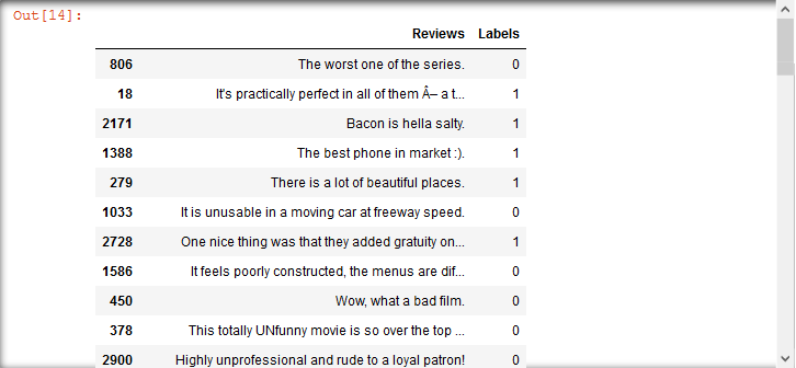
Summary statistics
import string df [ 'Word Count' ] = [ len ( review . split ()) for review in df [ 'Reviews' ]] df [ 'Uppercase Char Count' ] = [ sum ( char . isupper () for char in review ) \ for review in df [ 'Reviews' ]] df [ 'Special Char Count' ] = [ sum ( char in string . punctuation for char in review ) \ for review in df [ 'Reviews' ]] 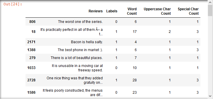
Word Count
positive_samples [ 'Discussion Count' ] . describe ()
count 1500.000000 hateful 11.885333 std 7.597807 min 1.000000 25% six.000000 fifty% 10.000000 75% 16.000000 max 56.000000 Proper name: Discussion Count, dtype: float64
negative_samples [ 'Word Count' ] . depict ()
count 1500.000000 mean xi.777333 std 8.140430 min 1.000000 25% six.000000 50% 10.000000 75% sixteen.000000 max 71.000000 Proper noun: Word Count, dtype: float64 Capital Character Count
positive_samples [ 'Capital letter Char Count' ] . draw ()
count 1500.000000 mean i.972667 std 2.103062 min 0.000000 25% 1.000000 50% 1.000000 75% 2.000000 max 17.000000 Proper noun: Uppercase Char Count, dtype: float64
negative_samples [ 'Capital Char Count' ] . describe ()
count 1500.000000 mean 2.162000 std 3.912624 min 0.000000 25% 1.000000 50% 1.000000 75% 2.000000 max 78.000000 Proper name: Uppercase Char Count, dtype: float64 Special Grapheme Count
positive_samples [ 'Special Char Count' ] . depict ()
count 1500.000000 mean two.140667 std 1.827687 min 0.000000 25% 1.000000 50% 1.500000 75% 3.000000 max nineteen.000000 Proper noun: Special Char Count, dtype: float64
negative_samples [ 'Special Char Count' ] . draw ()
count 1500.000000 mean two.165333 std one.661276 min 0.000000 25% 1.000000 50% ii.000000 75% iii.000000 max 14.000000 Name: Special Char Count, dtype: float64
from collections import Counter def getMostCommonWords ( reviews , n_most_common , stopwords = None ): # param reviews: column from pandas.DataFrame (e.grand. df['Reviews']) #(pandas.Serial) # param n_most_common: the top n most common words in reviews (int) # param stopwords: list of stopwords (str) to remove from reviews (listing) # Returns list of n_most_common words organized in tuples equally #('term', frequency) (list) # flatten review column into a list of words, and set each to lowercase flattened_reviews = [ word for review in reviews for word in \ review . lower () . split ()] # remove punctuation from reviews flattened_reviews = [ '' . join ( char for char in review if \ char not in cord . punctuation ) for \ review in flattened_reviews ] # remove stopwords, if applicable if stopwords : flattened_reviews = [ word for word in flattened_reviews if \ word not in stopwords ] # remove whatsoever empty strings that were created by this process flattened_reviews = [ review for review in flattened_reviews if review ] return Counter ( flattened_reviews ) . most_common ( n_most_common )
import nltk nltk . download ( 'stopwords' ) from nltk.corpus import stopwords stopwords.words('english'). Now lets get a quick snapshot of the 2 classes, with and without stopwords. First, for the positive course:Positive Grade with Stopwords
getMostCommonWords ( positive_samples [ 'Reviews' ], 10 )
[( 'the', 989 ), ( 'and', 669 ), ( 'a', 466 ), ( 'i', 418 ), ( 'is', 417 ), ( 'this', 326 ), ( 'it', 311 ), ( 'of', 308 ), ( 'to', 305 ), ( 'was', 257 )] Positive Course without Stopwords
getMostCommonWords ( positive_samples [ 'Reviews' ], 10 , stopwords . words ( 'english' ))
[( 'dandy', 198 ), ( 'expert', 174 ), ( 'picture', 98 ), ( 'phone', 86 ), ( 'motion picture', 83 ), ( 'one', 76 ), ( 'best', 63 ), ( 'well', 61 ), ( 'food', threescore ), ( 'place', 58 )] Negative Class with Stopwords
getMostCommonWords ( negative_samples [ 'Reviews' ], 10 )
[( 'the', 951 ), ( 'i', 469 ), ( 'and', 460 ), ( 'a', 420 ), ( 'to', 361 ), ( 'it', 354 ), ( 'is', 336 ), ( 'this', 313 ), ( 'of', 313 ), ( 'was', 312 )] Negative Class without Stopwords
getMostCommonWords ( negative_samples [ 'Reviews' ], x , stopwords . words ( 'english' ))
[( 'bad', 96 ), ( 'movie', 94 ), ( 'phone', 76 ), ( 'dont', seventy ), ( 'like', 67 ), ( 'i', 67 ), ( 'food', 64 ), ( 'time', 61 ), ( 'would', 57 ), ( 'film', 57 )] Vectorization: Translating from English to Computer-Speak
[ 'the true cat is black', 'I am cat like black true cat', 'the emu is black' ]
array([[ 0, i, one, 0, 1, 0, 1 ], [ 1, i, 2, 0, 0, 1, 0 ], [ 0, 1, 0, i, 1, 0, 1 ]], dtype =int64)
{ 'am': 0, 'black': 1, 'cat': 2, 'emu': iii, 'is': 4, 'like': 5, 'the': vi }
assortment([[ 0. , 0.409, 0.527, 0. , 0.527, 0. , 0.527], [ 0.463, 0.274, 0.704, 0. , 0. , 0.463, 0. ], [ 0. , 0.373, 0. , 0.632, 0.480, 0. , 0.480]])
from sklearn.feature_extraction.text import TfidfVectorizer vectorizer = TfidfVectorizer () bow = vectorizer . fit_transform ( df [ 'Reviews' ]) labels = df [ 'Labels' ]
len ( vectorizer . get_feature_names ())
vectorizer = TfidfVectorizer ( min_df = 15 ) bow = vectorizer . fit_transform ( df [ 'Reviews' ]) len ( vectorizer . get_feature_names ())
from sklearn.feature_selection import SelectKBest , chi2 # select the 200 features that have the strongest correlation to a class from the # remaining 308 features. selected_features = \ SelectKBest ( chi2 , k = 200 ) . fit ( bow , labels ) . get_support ( indices = True )
vectorizer = TfidfVectorizer ( min_df = 15 , vocabulary = selected_features ) bow = vectorizer . fit_transform ( df [ 'Reviews' ]) bow
3000x200 sparse matrix of type '<class 'numpy.float64'>' with 11889 stored elements in Compressed Sparse Row format Splitting the Dataset: The Railroad train and Test Sets
from sklearn.model_selection import train_test_split X_train , X_test , y_train , y_test = train_test_split ( bow , labels , test_size = 0.33 ) The Classifier
from sklearn.ensemble import RandomForestClassifier as rfc
classifier = rfc () classifier . fit ( X_train , y_train ) classifier . score ( X_test , y_test ) Hyperparameter Optimization: Maximizing Performance
from sklearn.model_selection import RandomizedSearchCV from scipy import stats classifier = rfc () hyperparameters = { 'n_estimators' : stats . randint ( 10 , 300 ), 'benchmark' :[ 'gini' , 'entropy' ], 'min_samples_split' : stats . randint ( ii , 9 ), 'bootstrap' :[ Truthful , False ] } random_search = RandomizedSearchCV ( classifier , hyperparameters , n_iter = 65 , n_jobs = 4 ) random_search . fit ( bow , labels )
optimized_classifier = random_search . best_estimator_ optimized_classifier . fit ( X_train , y_train ) optimized_classifier . score ( X_test , y_test ) Results analysis
optimized_classifier . fit ( bow , labels ) our_negative_sentence = vectorizer . transform ([ 'I hated this production. It is \ not well designed at all, and it broke into pieces equally shortly as I got it. \ Would non recommend anything from this company.' ]) our_positive_sentence = vectorizer . transform ([ 'The movie was superb - I was \ on the edge of my seat the entire fourth dimension. The acting was first-class, and the \ scenery - my goodness. Sentinel this film at present!' ]) optimized_classifier . predict_proba ( our_negative_sentence )
assortment([[ 0.84355159, 0.15644841]])
optimized_classifier . predict_proba ( our_positive_sentence )
assortment([[ 0.11276455, 0.88723545]])
our_slightly_negative_sentence = vectorizer . transform ([ "The product was okay. \ I've ordered amend in the by, and overall, I'd probably recommend a unlike \ product line if you lot're new to these. The company is good, though, and they do \ have some first-class products. This product isn't actually i of them." ]) our_slightly_positive_sentence = vectorizer . transform ([ "The dorsum finish of the phone \ barbarous off upon delivery - a attestation to its cheap, plastic build. After six months \ of connected employ, however, I must say this product is incredible bang for your \ buck. It's pretty good, and you'd be difficult pressed to find something similar for \ this matter'due south low cost." ]) optimized_classifier . predict_proba ( our_slightly_negative_sentence )
assortment([[ 0.1031746, 0.8968254]])
optimized_classifier . predict_proba ( our_slightly_positive_sentence )
array([[ 0.6274093, 0.3725907]])
optimized_classifier . fit ( X_train , y_train ) correctly_classified = {} incorrectly_classified = {} for index , row in enumerate ( X_test ): probability = optimized_classifier . predict_proba ( row ) # become the location of the review in the dataframe. review_loc = y_test . alphabetize [ index ] if optimized_classifier . predict ( row ) == y_test . iloc [ index ]: correctly_classified [ df [ 'Reviews' ] . loc [ review_loc ]] = probability else : incorrectly_classified [ df [ 'Reviews' ] . iloc [ review_loc ]] = probability Misclassified Samples
for review , score in incorrectly_classified . items (): print ( '{}: {}' . format ( review , score [ 0 ])) print ( '-----' )
That's right....the ruby velvet cake.....ohhh this stuff is and then good.: [0.50008503 0.49991497] ----- Once more, no plot at all. : [0.52423469 0.47576531] ----- Doesn't do the chore.: [ 0.6735395 0.3264605] ----- Penne vodka excellent!: [ 0.84047619 0.15952381] ----- The Han Nan Chicken was as well very tasty.: [ 0.54190239 0.45809761] ----- I establish the product to be easy to set upwards and utilize.: [ 0.5163053 0.4836947] ----- Nosotros have gotten a lot of compliments on it.: [ 0.3891861 0.6108139] ----- I institute this production to be waaay too big.: [ 0.37018315 0.62981685] ----- i felt insulted and disrespected, how could you talk and judge another man being like that?: [ 0.46852324 0.53147676] ... Correctly Classified Samples
for review , score in correctly_classified . items (): impress ( '{}: {}' . format ( review , score [ 0 ])) impress ( '-----' )
The final three times I had lunch here has been bad.: [ 0.89693878 0.10306122] ----- Our waiter was very attentive, friendly, and informative.: [ 0.18739607 0.81260393] ----- The coaction betwixt Martin and Emilio contains the aforementioned wonderful chemistry we saw in Wall Street with Martin and Charlie. : [ 0.20173847 0.79826153] ----- Get To Identify for Gyros.: [ 0.39796863 0.60203137] ----- Everything was fresh and delicious!: [ 0.04166667 0.95833333] ----- I beloved this cablevision - it allows me to connect whatsoever mini-USB device to my PC.: [ 0.08222789 0.91777211] ----- This is simply the BEST bluetooth headset for audio quality!: [ 0.06885359 0.93114641] ... Determination
Source: https://www.tensorscience.com/nlp/sentiment-analysis-tutorial-in-python-classifying-reviews-on-movies-and-products
0 Response to "Positive and Negative Reviews About Heaven Is for Real"
Postar um comentário